


A medical expert on NakedCapitalism, recently mentioned an example of his kid’s teacher setting a mathematical equation to estimate two unknowns [a]: something most numerate people will recognise as impossible. While one teacher mistake isn’t scary, the fact our statistics programs just choose an arbitrary solution when encountering this phenomenon regularly in fields as diverse as Randomised Controlled Trials (RCTs) through to political polling is very concerning.
To help maximise engagement, I will illustrate this using a hypothetical political opinion poll. However, I will go on to explain how people in “hard sciences” should be equally worried, if not more so, since the problem is less well known among the RCT community, and will offer guidance to help practitioners.
I was once told “explain what you’re going to teach, teach it, then explain what you taught” so I’ll try to broadly follow that.
Here is is fundamental issue:
A pattern of “respond/not responded) (two percentages) or a pattern of votes across five political parties (a+b+c+d+e=100) is explainable by an infinite number of “mean affinities” (often interpreted as party loyalties but could be in a trials sense, “average response on some unobservable scale” which is the “true beta”) and “variances” (how variable you might be in giving the core response). Just so we are on the same page, although sigma (the standard deviation) when squared equals the variance, is usually referred to in equations, for reasons lost to the mists of time, choice modellers didn’t like to quote what the equation spits out: beta/sigma. Thinking of a large quoted value as a possibly large beta or a small sigma seemed to confuse some early people (because it is the MEAN divided by the VARIANCE) so they decided to work with the INVERSE of sigma, lamda, interpretable as “how consistent you are”. So small sigma (small variance) is high lamda (high consistency in response. So all this stuff is because what the program gives you is a large parameter which might be due to a large beta or a small sigma and you have NO IDEA which: high affinity (true beta) or low variance (how consistency – true lamda). The program gives you one times the other and you have NO IDEA what is driving the value.
What’s the problem with the likelihood function?
The likelihood function for logit models and the one for probit models[a] is an equation where the “beta” estimates it spits out are NOT in fact the true betas (measures of how strong the effect of each variable is in explaining your observed outcome). This is where the classic “two variables, one equation” problem comes in.
So, when choosing a political party, each beta is in a fact a perfect mix (“confound”) of two things:
How strong is the support for each candidate?
How certain/consistent is an individual person’s support for each candidate?
These are multiplied together so you have literally no way to split them back up into their two parts. In other words, the first is a measure of “how much you identify with a candidate” (mean – the “true beta”, somewhat confusingly typically labelled V in the math equations since V is often used to represent utility of a proxy for it) whilst the second is a measure of “how often you’ll stick with the candidate” (inverse of the variance which you can think of as consistency which mathematically we represent as lamda – as I said above, this is the INVERSE of sigma (the standard deviation) so measure CONSISTENCY NOT VARIANCE – high consistency (low variance) is generally GOOD).
Your preferred statistical package cannot separate beta from lamda – it can only give beta multiplied by lamda when it uses the (log)likelihood [b]. So it simply assumes that lamda is one: all the reported effects are implied to be true betas when they are not – they are true beta multiplied by lamda. For every person and every choice/medical intervention. To see how this might give you a very misleading picture about “what is going on” I’ll use a UK constituency election example. However, “medical brain trust” people bear with me, as I’ll go on to show how dangerous this statistical practice can be in the context of clinical studies including possibly the rush to get mRNA vaccines to market.
What’s the problem with the likelihood function?
The likelihood function for logit models and the one for probit models[a] is an equation where the “beta” estimates it spits out are NOT in fact the true betas (measures of how strong the effect of each variable is in explaining your observed outcome). This is where the classic “two variables, one equation” problem comes in.
So, when choosing a political party, each beta is in a fact a perfect mix (“confound”) of two things:
How strong is the support for each candidate?
How certain/consistent is an individual person’s support for each candidate?
In other words, the first is a measure of “how much you identify with a candidate” (mean – the “true beta”, somewhat confusingly typically labelled V by economists) whilst the second is a measure of “how often you’ll stick with the candidate” (inverse of the variance which you can think of as consistency which mathematically we represent as lamda).
Your preferred statistical package cannot separate beta from lamda – it can only give beta multiplied by lamda when it uses the (log)likelihood [b]. So it simply assumes that lamda is one: all the reported effects are implied to be true betas when they are not. For every person and every choice/medical intervention. To see how this might give you a very misleading picture about “what is going on” I’ll use a UK constituency election example. However, “medical brain trust” people bear with me, as I’ll go on to show how dangerous this statistical practice can be in the context of clinical studies including possibly the rush to get mRNA vaccines to market.
An example using a very “middle England” constituency
Here are some hypothetical numbers that look like results from a UK opinion poll conducted in a “middle England” constituency. However, the reader should try to keep in mind that they are actually the “internal tendency to support each party for one individual, called Jo”. Jo simply said “conservative” but these are her internal percentages. The reasons for this will become clear. Until mid 2024 the Conservatives were the main right-wing party of government (somewhat like the US Republicans), Reform UK were attacking them from the right on issues like keeping out of the EU and DEI (MAGA type messages). Labour was supposedly centre-left (US Democrats) with a very mixed attitude toward the EU, whilst the Lib Dems and Green positioned themselves as forces to the middle or left who wanted back into the EU, some of whom could be quite libertarian but with a strong “left-wing tilt amongst Greens anyway”.
These percentages are effectively our “y” dependent variables in a logit or probit model based on likelihoods: what set of betas (our independent variables indicating “level of party affinity”) is most likely to give these percentages. Yet unless you read the appendix to these models in the manuals to a program like Stata, or work in one of only a few fields that encourage you to think about what the individual is doing (mathematical psychology or n-of-1 RCTs) then you won’t realise that what you are getting are not betas, but betas_times_lamdas! The program has decided “ok set lamda to be one” encouraging you to think that all of these levels of support came from innate levels of strength of support for each party, rather than any consistency (or lack thereof) in support. Putting out misinformation about rivals to reduce consistency of support for them is a great way to artificially boost your percentage of the vote if you realise you can’t boost your “real beta – strength of support” easily.
A brief delve into the weeds “how an individual responds” in terms of the mathematics
I won’t cause people’s eyes to glaze over with a complete discussion of the likelihood function that translates “proportions” into “pseudo-betas” (pseudo because they’re confounded with lamdas). Somewhat surprisingly, it wasn’t until the mid 1980s that the theoretical proof of the likelihood function doing this was published by Yatchew and Griliches[1][c].
I’ll simply use the crucial bit of the likelihood exploited by the field of choice modelling (and clinical trials but I’ll come to those shortly). In areas like academic marketing, random utility theory is used[2]. This was developed by Thurstone in 1927 and was at its heart a signal-to-noise way of conceptualising human choice (probably why mainstream economists generally dislike it: people are meant to conform to things like transitivity so the idea they might make mistakes is anathema). However, Thurstone was actually thinking at the level of the individual participant (think of our voter called Jo): how often they chose item i over some set of items y=1,2,…. tells you how much they value i over any other member of the set of y-1. Hence the core equation:
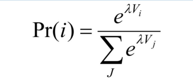
This is not as scary as it looks. The probabilities (observed frequencies) are the left hand side and the numbers your favourite stats program gives you for your (in this case five) parties are the lamda-times-V. Perhaps you’ve spotted the problem. It cannot separate V from lamda so it sets lamda to be one (it “normalises it”). So ALL the variation in those percentages above are explained by “betas” which are in fact a perfect mix of V (the true affinity/strength) and lamda (consistency). Also, it is not exactly how clinical trials work but the problem at their heart is identical, as described in reference 1.
In short, the “vote shares” (probabilities) in Table 1 below are the left hand side. These need to be explained by five “lamda-Vs”.The V is the utility (“true affinity score or utility”). So if all affinity scores were zero (“meh to every party”) then each probability would be exp(0)=1 divided by the five exponents (each being one) so 1/5=20%. So that figures. As the V (true affinity score) increases for a given Party, then its contribution to the total (the numerator over the denominator) increases. Here’s what Stata et al do:
Table 1: How Stata interprets percentages to give “betas”
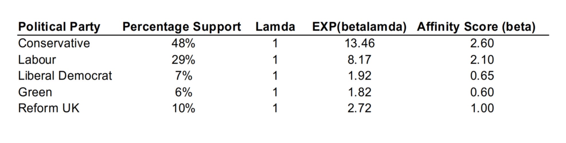
The reader who wants to check can simply calculate the exponential of (affinity score times lamda) for each party, to give the figure in column 4, The sum of the figures in column 4 is 28.09. 13.46 is 48% of 28.09, which is the Conservative percentage, and so on. Note, once again, that the stats package would not normally know these affinity scores (the “true betas”). It would use the logit function to translate the column 2 percentages into the column 4 figures from part 1, but by assuming lamda=1 for every party would get the affinity scores in final column.
So, according to pollsters, we have numbers purporting to show Jo’s level of affinity with each party. As the raw “percentages” suggest, she feels most aligned with the Conservatives, then Labour, with Reform UK, the Lib Dems and Greens in that order a distant 3rd, 4th and 5th. However, this could just as easily be a potentially deeply misleading characterisation of her views.
Table 2 shows an alternative set of numbers that produces the EXACT SAME PERCENTAGES.
Table 2: Re-interpreting percentages as if Jo were “Old School anti-EU Labour”
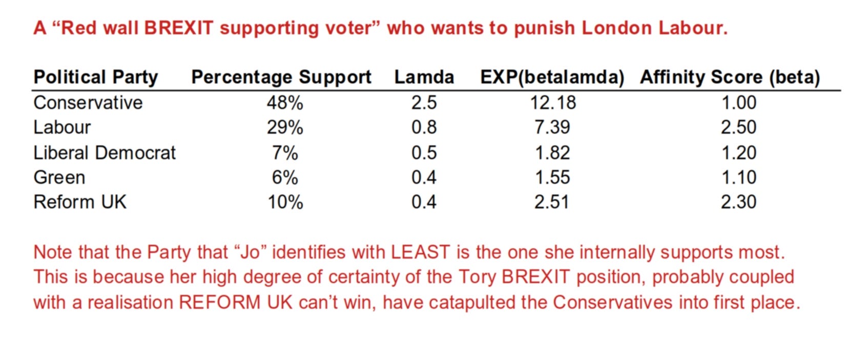 Again, we use Jo’s “internal pseudo-percentage support levels” in the standard logit equation to work out what her “V times lamdas” are. Again, I’m “being God” and knowing what her levels of consistency (her lamdas) are for every party. Again, I can get “correct” levels of her support (affinity scores) for each party. I simply use the “percentages”, together with my “god-like knowledge of her certainty/consistency” with the logit equation to solve for “affinity scores”. These are our “real betas” presented in the last column. THESE are true levels of “intrinsic support” for each party. Turns out she’s like many people who started going Labour in 2024. Jo’s low internal percentage support for Reform might simply reflect that the she’s far more certain about the establishment Conservatives continuing to deliver on BREXIT than the somewhat populist Reform UK.
Table 3: Re-interpreting percentages as if Jo were “Conservative with unclear EU views”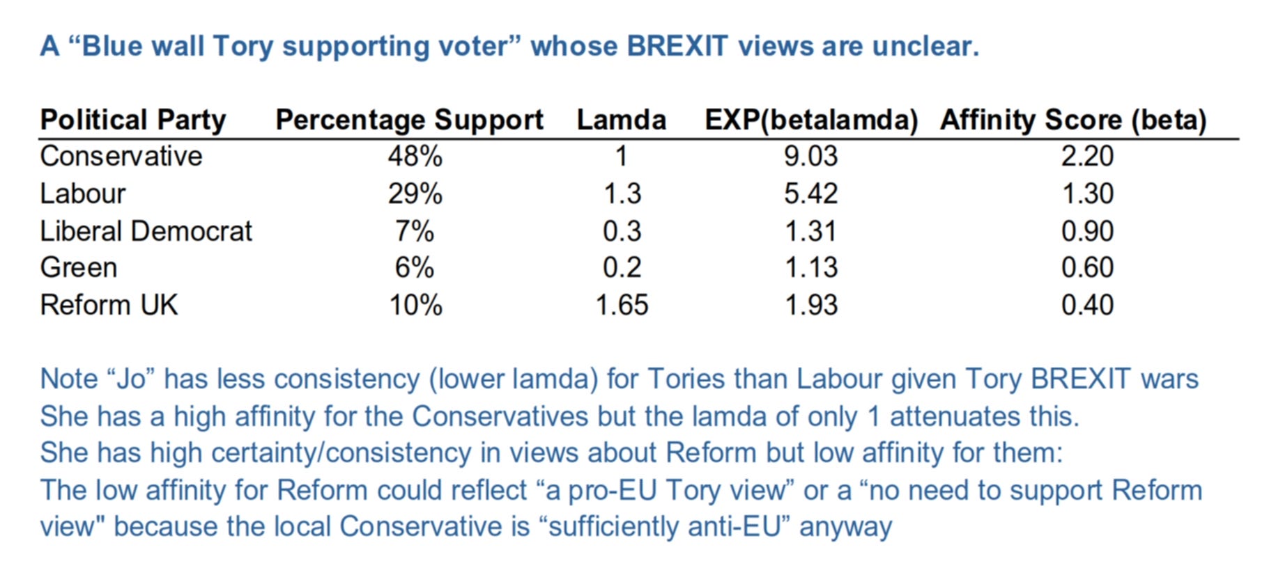
So Stata and other programs assumed that the contents of Table 1 represented Jo’s thought process. I’ve made up two completely different scenarios (Table 2 and 3) that give the same percentages. If that makes you worried then you should be. In the tables above I “played God” by knowing the true split between V and lamda but pollsters DO NOT.
These percentages conceal some crucial aspects of Jo’s thinking
So……“Jo types” could, via different lamdas, be people who were the classic “Blue Wall Conservative” who could have voted either way in the BREXIT referendum and who only had truck with Labour and the Conservatives and very possibly the Lib Dems? Or that their data were equally consistent with a person resident in part of the “broken-and-now-rebuilt-red-wall” in the Midlands who actually were “old school Labour” and who lent support to the right because she thought Labour were in the pockets of the EU and wanted to kick the establishment in the teeth? Both explanations are possible from these data.
So far I’ve showed how a logit model (the workhorse of political voting models) interpreted observed percentage levels of support. It should be noted that reputable pollsters apply sampling weights to ensure that they have interviewed sufficient supporters of every party of interest. Under-representing certain parties, or those who actually will go out and vote come election day, will immediately lead to a bad prediction.
Note that the clever psephologist who either had a SECOND dataset that had some function of the affinity scores in there, or used a lot of qualitative insights into the local constituency, might alter the lamdas to get “more correct” affinity scores and thereby tease out what is really going on. If you hear the term “Multi-level Regression and Post-stratification” then that’s their fancy way of saying they’re drawing on auxiliary information in order to try to avoid the traps I’ve described above.
What does this all mean for our psephologist trying to tell us what is going on out there?
In an era of increasingly sophisticated marketing and targeting and Artificial Intelligence being used to confuse people, the ones in the first group – supposedly “strong” Tories – might not turn out to vote if their levels of uncertainty are ramped up via social media lies. Conversely, other parties can reduce the Tory vote if they know “Tory tribalism is low” and the Tories are doing well merely because these other parties are not producing clear messages that cause voters’ certainty regarding policy to increase.
Polling implications
I cheated by “knowing” how much our hypothetical voter Jo identified with each party. However, I showed that some realistic values, given UK experience, could mean her “relative levels of party support” are consistent with various profoundly different types of constituency result in the UK.
This should make psephologists and statisticians very wary. “Turnout” can no longer be used as their “get out of jail free card” when they predict wrongly.
Researchers in discrete choice modelling know full well already that they cannot aggregate Jo’s data with other survey participants UNTIL AND UNLESS YOU HAVE NETTED OUT ANY DIFFERENCES IN THEIR CONSISTENCY (VARIANCES). Crucially, the Central Limit Theorem does NOT apply here [1]
Researchers must own up to the fact that EVERY opinion poll is an equation with two unknowns and therefore insoluble.
YouGov grasped the nettle in 2017 by administering a second survey to try to get a handle on “intrinsic attitudes”. That “alternative model” was the only “official model” to correctly predict that Prime Minister Theresa May was about to lose her overall majority in Parliament, having called a surprise General Election. (By chance I had a political national survey in field at that time and also predicted this – I made money at the bookies but no media were interested.)
So how might this play out in Medicine?
As with all “first attempts” at illustrating the intuition behind some quite heavy duty concepts, I’ve still had to make some simplifications: the “random utility equation” is merely a (I hope) fairly easily understood subset of the likelihood function for logit models. I hope that what I’ve ended up writing at least helps the readers who have asked me for “the intuition” to feel that they get a better handle on why “one-shot” percentages can be so dangerous when it comes to interpreting “what’s going on at the fundamental level of THE INDIVIDUAL HUMAN”.
YOU SEE A JPEG WHEN YOU REALLY NEED TO SEE AN MPEG.
The paradigm I worked in for 20 years – Random Utility Theory – was all about modelling an individual human. Treating the “errors” not as some “bad thing” but as simply a characteristic of our decisions can be incredibly empowering when it comes to quantifying what we really value. To be colloquial – signal vs noise tells us a LOT and gives us proper NUMBERS.
First of all, it is important to recognise that “variance” in responses quoted from RCTs etc refers to “variability between individuals” NOT “variability within a given individual” (since as I have shown above, a “one shot” study – like an RCT – cannot shed light on this). So let me give you something to think about. Suppose two patients both respond in a one-shot RCT to the active treatment. However, suppose, if we’d done the trial 16 times (8 times receiving the active treatment, 8 times the placebo, with adequate washout periods between rounds) we observed that patient A responded all 8 times whilst patient B respondent 5 out of 8 times. You’d probably want to know if there is something going on to explain this difference.
Patients in RCTs typically are heavily screened to ensure nobody with a potentially confounding condition might be enrolled which could compromise the results. But suppose there is an unobserved difference between patients that causes the 8/8 people to be mixed in with the 5/8 people? Yatchew and Grilisches proved that you CANNOT aggregate these two groups to get an unbiased estimate of the “true beta – strength of effect” unless you “net out” the differences in consistency first. But if your painstaking attempts to ensure a very homogeneous sample do not, in fact, do anything to address this then your work is all in vain.
I’m no geneticist but I can hypothesise reasons why the 5/8 persons are allowed to be aggregated with the 8/8 people if you’ve rushed early stages of drug development. Suppose a combination of 3 genes ensures you’ll ALWAYS respond to the treatment, but having only 1 or 2 of the 3 gives you only a partial response (5 out of 8 times). This touches upon the issue of the fast rollout of the mRNA vaccines: not that they are necessarily bad, but merely that you should never rush things. It is the early stage trials with genetic tests that offers one potential way to separate the “5/8” people from the “8/8” people and might give you insights WHY. Because you really don’t want to “move fast and break things” and have no idea why some people are consistently responding to something whilst others, for reasons unknown, have inconsistent responses over time (or worse, suffer specific side effects).
The solution?
When I was doing my PhD (in understanding ways to analyse cluster RCTs – where you must randomise, for example schools, or whole hospitals, to avoid contamination of the two arms) I had to learn Fortran if I were to get the simulations done in 3 years. A colleague learnt Fortran with me: but for her, it was to enable simulations “going in the opposite direction” – learning how the individual might display inconsistency in response. Her work contributed to the field of the “n-of-1 trial”. This is a kind of trial that recognises that consistency might vary across patients and you must adjust for it. Unfortunately that type of trial never really took off: those trials are resource intensive and obviously expensive and when the statistical establishment (with some exceptions) don’t even recognise the weakness in their models, you’re not going to change the paradigm.
But to any of the “medical brain trust” who made it this far – if you see stuff that “seems off” given what evidence based medicine has taught you, maybe the problem is the trial, not with you. Judgment can be our best friend. I spent 15 years accumulating it in recognising patterns of the “betas” spit out by Stata and why they “did not compute”.
What did I just try to teach?
An RCT or poll is a jpeg. You need an mpeg. Just knowing relative positions is NOT enough. You need to know “intrinsic ability” together with “consistency”. Certain studies will tell you “there are segments with different levels of ability” and/or “consistency”. However, if you are to ACT upon this you really must have done enough work to ensure you understand what is DRIVING (in)consistency, otherwise you might get a nasty shock you run a study in a new sample.
NOTES:
[a] https://www.nakedcapitalism.com/2025/05/thinking-being-offloaded-to-ai-even-in-elite-medical-programs.html#comment-4219558
[b] Daniel McFadden won the “pseudo Economics Nobel” and is one of only about 3 people I think deserved it. Whether he knew already that TWO datasets were required to design the BART in the Bay Area or just wanted a 2nd “real usage” dataset to calibrate his model, he clearly solved the problem by having two equations for two unknowns.
[c] Probit models are difficult when the number of outcomes is above 2 so I’ll gloss over these but the principle is the same. Since the probit function, when graphed, is so similar to the logit, many practitioners just use the logit to avoid the estimation complications of the probit.
Bibliography
[1] https://www.jstor.org/stable/1928444?origin=crossref: Adonis Yatchew and Zvi Griliches. Specification Error in Probit ModelsThe Review of Economics and Statistics Vol. 67, No. 1 (Feb., 1985), pp. 134-139
[2] Thurstone LL. A law of comparative judgment. Psychological Review, 34, 273-286 (1927).


